Aitoff with boinor for plotting celestial bodies

Visualizing celestial positions on an all-sky map is essential for understanding the spatial distribution of objects in the sky. The Aitoff projection is a modified azimuthal map projection that displays the entire celestial sphere in a single view, making it ideal for astronomical visualization.

boinor provides the AitoffPlotter class for creating all-sky maps in J2000 equatorial coordinates (right ascension and declination). This projection is particularly useful for:

• Visualizing the positions of planets, moons, and spacecraft

• Understanding the distribution of celestial objects across the sky

• Planning observations and mission trajectories

• Analyzing the geometry of interplanetary missions

The Aitoff projection operates in J2000 equatorial coordinates without Earth-orientation or horizon effects, making it suitable for inertial sky visualization. This means the map shows positions as they would appear from an inertial reference frame, not as seen from Earth’s surface at a specific location.

Basic usage

Let’s start with a simple example plotting points using right ascension and declination coordinates:

from astropy import units as u
from astropy.time import Time
import numpy as np


from boinor.plotting import AitoffPlotter

The AitoffPlotter class can be initialized with various options. The simplest usage creates a plotter with the current epoch:

# Create plotter with current epoch
plotter = AitoffPlotter(epoch=Time.now())

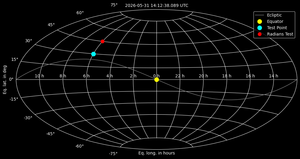
# Plot a point at RA=0h, Dec=0deg (celestial equator)
plotter.plot_ra_dec(ra=0*u.hourangle, dec=0*u.deg, label="Equator", color="yellow", markersize=10)

# Plot a point at RA=6h, Dec=30deg
plotter.plot_ra_dec(ra=6*u.hourangle, dec=30*u.deg, label="Test Point", color="cyan", markersize=10)

# Plot using radians directly
plotter.plot_ra_dec(ra=np.pi/2, dec=np.radians(45), label="Radians Test", color="red", markersize=8)

# Display the plot
plotter.show()

The plot_ra_dec method accepts coordinates in various formats:

• Astropy quantities (e.g., 0*u.hourangle, 30*u.deg)

• Radians (as floats or numpy arrays)

• Any unit that Astropy can convert to radians

Customizing the plot

You can customize the appearance of the sky map by providing custom matplotlib axes, figure size, and style:

from matplotlib import pyplot as plt

# Create custom figure and axes
fig, ax = plt.subplots(figsize=(15, 9), subplot_kw={"projection": "aitoff"})

# Create plotter with custom axes
plotter = AitoffPlotter(
    epoch=Time.now(),
    ax=ax,
    style="default",  # Use default style instead of dark_background
    show_ecliptic=True  # Show ecliptic reference line
)

# Plot multiple points
# Origin: RA=0°, Dec=0° (celestial equator at vernal equinox)
plotter.plot_ra_dec(ra=0*u.deg, dec=0*u.deg, label="Origin", color="blue", markersize=10)
# NE Quadrant: RA=90° (6h), Dec=45° (northeast quadrant of sky)
plotter.plot_ra_dec(ra=90*u.deg, dec=45*u.deg, label="NE Quadrant", color="green", markersize=10)
# South: RA=180° (12h), Dec=-30° (southern declination)
plotter.plot_ra_dec(ra=180*u.deg, dec=-30*u.deg, label="South", color="orange", markersize=10)

plotter.show()

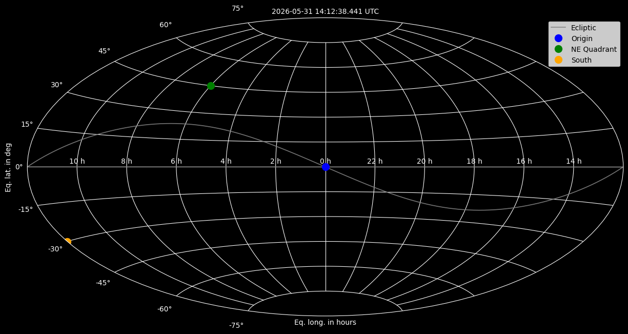
The ecliptic reference line (shown in gray) represents the plane of Earth’s orbit around the Sun, projected onto the celestial sphere. This is useful for understanding the positions of planets, which generally lie near the ecliptic.

Using SPICE ephemeris data

For more accurate positions of Solar System bodies, you can use SPICE kernels with the plot_spice_position method. This requires the spiceypy package and appropriate SPICE kernels.

First, you need to download SPICE kernels. The following commands show how to download the necessary kernels (commented out as these are large files):

# Download SPICE kernels (commented out - these are large files)
!curl https://naif.jpl.nasa.gov/pub/naif/generic_kernels/lsk/naif0012.tls --create-dirs -o kernels/lsk/naif0012.tls
!curl https://naif.jpl.nasa.gov/pub/naif/generic_kernels/spk/planets/de432s.bsp --create-dirs -o kernels/spk/de432s.bsp
!curl https://naif.jpl.nasa.gov/pub/naif/generic_kernels/pck/gm_de440.tpc --create-dirs -o kernels/pck/gm_de440.tpc
# !curl https://naif.jpl.nasa.gov/pub/naif/generic_kernels/spk/satellites/sat415.bsp -o kernels/spk/sat415.bsp

  % Total    % Received % Xferd  Average Speed   Time    Time     Time  Current
                                 Dload  Upload   Total   Spent    Left  Speed
  0     0    0     0    0     0      0      0 --:--:-- --:--:-- --:--:--     0
curl: (60) SSL certificate problem: unable to get local issuer certificate
More details here: https://curl.se/docs/sslcerts.html

curl failed to verify the legitimacy of the server and therefore could not
establish a secure connection to it. To learn more about this situation and
how to fix it, please visit the web page mentioned above.
  % Total    % Received % Xferd  Average Speed   Time    Time     Time  Current
                                 Dload  Upload   Total   Spent    Left  Speed
  0     0    0     0    0     0      0      0 --:--:-- --:--:-- --:--:--     0
curl: (60) SSL certificate problem: unable to get local issuer certificate
More details here: https://curl.se/docs/sslcerts.html

curl failed to verify the legitimacy of the server and therefore could not
establish a secure connection to it. To learn more about this situation and
how to fix it, please visit the web page mentioned above.
  % Total    % Received % Xferd  Average Speed   Time    Time     Time  Current
                                 Dload  Upload   Total   Spent    Left  Speed
  0     0    0     0    0     0      0      0 --:--:-- --:--:-- --:--:--     0
curl: (60) SSL certificate problem: unable to get local issuer certificate
More details here: https://curl.se/docs/sslcerts.html

curl failed to verify the legitimacy of the server and therefore could not
establish a secure connection to it. To learn more about this situation and
how to fix it, please visit the web page mentioned above.

Once kernels are downloaded, you can load them and plot celestial bodies:

import spiceypy
import glob

# Load SPICE kernels
kernel_paths = glob.glob("kernels/**/*")
spiceypy.furnsh(kernel_paths)

# Create plotter
plotter = AitoffPlotter(epoch=Time.now())

# Plot Sun using NAIF ID (10 = Sun)
plotter.plot_spice_position(
    target=10,  # Sun NAIF ID
    observer=399,  # Earth NAIF ID
    label="Sun",
    color="yellow",
    markersize=20
)

# Plot Saturn using NAIF ID (699 = Saturn)
#plotter.plot_spice_position(
#    target=699,  # Saturn NAIF ID
#    observer=399,  # Earth NAIF ID
#    label="Saturn",
#    color="tab:orange",
#    markersize=15
#)

# Display
plotter.show()

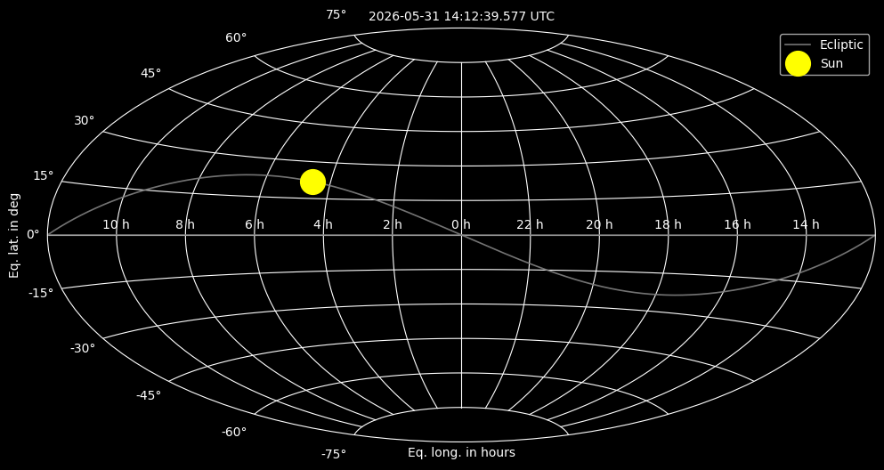
The plot_spice_position method automatically converts SPICE Cartesian coordinates to right ascension and declination, making it easy to visualize the positions of any body for which SPICE kernels are available.

Analysis example: Geometric vs. Apparent positions

When computing positions of celestial bodies, there are two important concepts:

• Geometric Position (abcorr="NONE"): The “true” instantaneous position where the object actually is at the specified time. This is the position in space without any corrections for the finite speed of light or observer motion.

• Apparent Position (abcorr="LT+S"): The position as it would appear to an observer, corrected for:

  • LT (Light Time): The time it takes light to travel from the object to the observer. Since light has finite speed, we see objects where they were when the light left them, not where they are now.

  • S (Stellar Aberration): The apparent shift in position due to the observer’s motion through space (similar to how raindrops appear to come from ahead when you’re moving).

As a sanity check, you can compare these two positions to understand the magnitude of relativistic effects. The following example demonstrates this analysis (commented out as it requires specific kernels and time):

import datetime


# Determine the current datetime
datetime_now = datetime.datetime.today()
datetime_now = datetime_now.strftime('%Y-%m-%dT%H:%M:%S')

# Convert to Ephemeris Time
et_now = spiceypy.utc2et(datetime_now)

# Print current time information
print(f"Current UTC time: {datetime_now}")
print(f"Ephemeris Time: {et_now}")

# Analysis for a specific target (e.g., Saturn) - commented out as it requires kernels
# target = 699  # Saturn Barycenter NAIF ID
# observer = 399  # Earth NAIF ID
# frame = "J2000"
#
# Geometric Position (NONE) - "True" instantaneous position
# pos_geo, _ = spiceypy.spkpos(target, et_now, frame, "NONE", observer)
#
# Apparent Position (LT+S) - Position corrected for light time and stellar aberration
# pos_app, _ = spiceypy.spkpos(target, et_now, frame, "LT+S", observer)
#
# Distance (Magnitude of the geometric vector)
# dist_km = spiceypy.vnorm(pos_geo)
# dist_au = spiceypy.convrt(dist_km, "KM", "AU")
#
# Angular Separation - The angular difference between geometric and apparent positions
# sep_rad = spiceypy.vsep(pos_geo, pos_app)
# sep_deg = sep_rad * spiceypy.dpr()
#
# def deg_to_dms(degrees):
#     d = int(degrees)
#     m_float = (degrees - d) * 60
#     m = int(m_float)
#     s = (m_float - m) * 60
#     return d, m, s
#
# d, m, s = deg_to_dms(sep_deg)
#
# print(f"--- Analysis for {datetime_now} UTC ---")
# print(f"Target: Saturn (NAIF ID {target}) | Observer: Earth (NAIF ID {observer})")
# print("-" * 40)
# print(f"Current Distance: {dist_km:,.2f} km")
# print(f"                  {dist_au:.6f} AU")
# print("-" * 40)
# print(f"Angular Error (Geo vs Apparent):")
# print(f"Degrees: {sep_deg:.8f}°")
# print(f"DMS:     {d}° {m}' {s:.4f}\"")

# Example output (computed for a typical date: 2026-01-18T05:00:34 UTC):
# Current UTC time: 2026-01-18T05:00:34
# Ephemeris Time: 821984503.1844143
# --- Analysis for 2026-01-18T05:00:34 UTC ---
# Target: Saturn (NAIF ID 699) | Observer: Earth (NAIF ID 399)
# ----------------------------------------
# Current Distance: 1,492,643,833.99 km
#                  9.977708 AU
# ----------------------------------------
# Angular Error (Geo vs Apparent):
# Degrees: 0.00476700°
# DMS:     0° 0' 17.1612"

Current UTC time: 2026-05-31T14:12:39
Ephemeris Time: 833508828.1849208

This analysis compares the geometric position (where Saturn actually is) versus the apparent position (where Saturn appears to be from Earth).

The results show:

• Distance: How far Saturn is from Earth (in km and AU)

• Angular Error: The angular separation between geometric and apparent positions, showing the effect of light time and stellar aberration

For distant objects like Saturn, the difference between geometric and apparent positions is typically small (on the order of arcseconds, ~0.005° in the example). However, this difference becomes more significant for:

• Closer objects (Mars, Venus)

• High-precision applications (spacecraft navigation, astrometry)

• Objects with high relative velocities

The AitoffPlotter uses apparent positions (abcorr="LT+S") by default in plot_spice_position, which is appropriate for realistic sky visualization.

Plotting multiple bodies

You can plot multiple celestial bodies on the same sky map to understand their relative positions:

# Load SPICE kernels
kernel_paths = glob.glob("kernels/**/*")
spiceypy.furnsh(kernel_paths)

plotter = AitoffPlotter(epoch=Time.now())

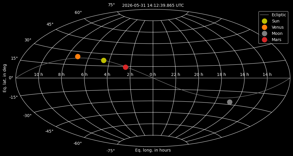
# Set a dictionary that lists some body names and the corresponding NAIF ID
# code. Mars has the ID 499, however the loaded kernels do not contain the
# positional information. We use the Mars barycentre instead
SOLSYS_DICT = {'SUN': 10, 'VENUS': 299, 'MOON': 301, 'MARS': 4}

# Each body shall have an individual color; set a list with some colors
BODY_COLOR_ARRAY = ['y', 'tab:orange', 'tab:gray', 'tab:red', 'tab:blue', 'tab:green']

# Iterate through the dictionary and plot each celestial body
for body_name, body_color in zip(SOLSYS_DICT, BODY_COLOR_ARRAY):

    # Plot the body using its NAIF ID
    plotter.plot_spice_position(
        target=SOLSYS_DICT[body_name],
        observer=399,  # Earth NAIF ID
        label=body_name.capitalize(),
        color=body_color,
        markersize=12
    )

plotter.show()

Understanding the coordinate system

The Aitoff projection in boinor uses J2000 equatorial coordinates:

• Right Ascension (RA): Measured eastward along the celestial equator from the vernal equinox, typically expressed in hours (0-24h) or degrees (0-360°)

• Declination (Dec): Measured north or south of the celestial equator, typically expressed in degrees (-90° to +90°)

The projection automatically handles coordinate conversions:

• Longitude values are converted to matplotlib’s expected format ([-π, π])

• Values are inverted to match standard sky map conventions where 0° longitude is on the left

• The ecliptic reference line is converted from ecliptic coordinates to equatorial coordinates using the mean obliquity of the ecliptic

This makes the AitoffPlotter ideal for visualizing positions in inertial space, without the complications of Earth’s rotation or local horizon effects.

Notes and limitations

• The Aitoff projection shows the entire celestial sphere, but objects near the poles may appear distorted

• The default style uses dark_background to simulate a night sky appearance

• SPICE kernel support requires the spiceypy package and appropriate kernels

• The projection assumes J2000 coordinates; for other epochs, proper coordinate transformations may be needed

• The ecliptic reference line uses the mean obliquity (23.439281°) for J2000; for high-precision applications, time-dependent obliquity should be used

References

• “High Accuracy” Orientation and Body-fixed Frames for the Moon and Earth

• Overview of Reference Frames and Coordinate Systems in SPICE

• SPICE Data (SPICE Kernels)

• SPICE-Lecture by Thomas Albin